Basic biolord pipeline

This code presents the pipeline of biolord for learning decoupled representations of known and unknown attributes in single-cell data.

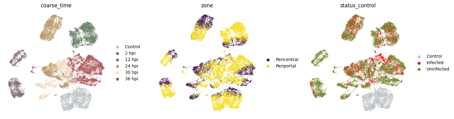
Here we train a Biolord model on the spatio-temporally resolved single cell atlas of the Plasmodium liver stage [AZLBH+22] to recover gene expression trends associated with infected state.

import pandas as pd
import numpy as np

import scanpy as sc
import biolord

import seaborn as sns
import matplotlib.pyplot as plt
import warnings
from scipy.stats import ttest_rel

warnings.simplefilter("ignore", UserWarning)

Setup the AnnData

adata = sc.read("adata_infected.h5ad", backup_url="https://figshare.com/ndownloader/files/39375713")

fig, axs = plt.subplots(1, 3, figsize=(15, 4))
for i, c in enumerate(["coarse_time", "zone", "status_control"]):
    sc.pl.umap(adata, color=[c], ax=axs[i], show=False)
    axs[i].set_axis_off()
plt.tight_layout()
plt.show()

By calling biolord.Biolord.setup_anndata() we set the supervised attributes used for disentanglement. The function takes as input:

• adata: the adata object for the setting.

• ordered_attributes_keys: the keys in obs or obsm defining ordered attributes.

• categorical_attributes_keys: the keys in obs defining categorical attributes.

biolord.Biolord.setup_anndata(
    adata,
    ordered_attributes_keys=None,
    categorical_attributes_keys=["time_int", "status_control", "zone"],
)

Run Biolord

Instantiate a Biolord model

We instantiate the model given the module_params.

These are parameters required to construct the model’s module, the various networks included in a Biolord model.

The parameters include standard architecture design values (e.g. width, depth, and latent dimension) and loss functon choices alongwith Biolord oriented parameters. The Biolord model parameters are:

• reconstruction_penalty: internal penalty term weighting the componenets of the reconstruction loss

• unknown_attribute_penalty: the penalty weight of the unknown_attribute magnitued in the final loss objective.

• unknown_attribute_noise_param: the std added to unknown attribute embedding

module_params = {
    "decoder_width": 1024,
    "decoder_depth": 4,
    "attribute_nn_width": 512,
    "attribute_nn_depth": 2,
    "n_latent_attribute_categorical": 4,
    "gene_likelihood": "normal",
    "reconstruction_penalty": 1e2,
    "unknown_attribute_penalty": 1e1,
    "unknown_attribute_noise_param": 1e-1,
    "attribute_dropout_rate": 0.1,
    "use_batch_norm": False,
    "use_layer_norm": False,
    "seed": 42,
}

model = biolord.Biolord(
    adata=adata,
    n_latent=32,
    model_name="spatio_temporal_infected",
    module_params=module_params,
    train_classifiers=False,
    split_key="split_random",
)

Train the model

To train the model we provide trainer_params. These are paramters which dictate the training regime, e.g., learning rate, weight decay and scheduler type.

trainer_params = {
    "n_epochs_warmup": 0,
    "latent_lr": 1e-4,
    "latent_wd": 1e-4,
    "decoder_lr": 1e-4,
    "decoder_wd": 1e-4,
    "attribute_nn_lr": 1e-2,
    "attribute_nn_wd": 4e-8,
    "step_size_lr": 45,
    "cosine_scheduler": True,
    "scheduler_final_lr": 1e-5,
}

model.train(
    max_epochs=500,
    batch_size=512,
    plan_kwargs=trainer_params,
    early_stopping=True,
    early_stopping_patience=20,
    check_val_every_n_epoch=10,
    num_workers=1,
    enable_checkpointing=False,
)

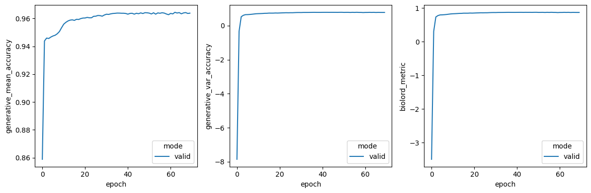
Epoch 70/500:  14%|█▍        | 70/500 [02:38<16:15,  2.27s/it, v_num=1, val_generative_mean_accuracy=0.964, val_generative_var_accuracy=0.776, val_biolord_metric=0.87, val_reconstruction_loss=18.8, val_unknown_attribute_penalty_loss=22, generative_mean_accuracy=0, generative_var_accuracy=0, biolord_metric=0, reconstruction_loss=18, unknown_attribute_penalty_loss=30.2]     
Monitored metric val_biolord_metric did not improve in the last 20 records. Best score: 0.874. Signaling Trainer to stop.

size = 4
vals = ["generative_mean_accuracy", "generative_var_accuracy", "biolord_metric"]
fig, axs = plt.subplots(nrows=1, ncols=len(vals), figsize=(size * len(vals), size))

model.epoch_history = pd.DataFrame().from_dict(model.training_plan.epoch_history)
for i, val in enumerate(vals):
    sns.lineplot(
        x="epoch",
        y=val,
        hue="mode",
        data=model.epoch_history[model.epoch_history["mode"] == "valid"],
        ax=axs[i],
    )

plt.tight_layout()
plt.show()

Recover infected signal

Compute expression predictions

Create a AnnData object with control cells

idx_source = np.where((adata.obs["split_random"] == "train") & (adata.obs["coarse_time"] == "Control"))[0]

adata_source = adata[idx_source].copy()

Use compute_prediction_adata() to obtain the expression predictions of control cells. The function takes as input:

• adata: the reference adata object to take attribute prediction categories.

• adata_source: the source adata to take initial state of the cells (i.e., the control cells).

• target_attributes: the attributes predictions are made with respect to (i.e., for target_attributes = ["status_control"] control cells will be evaluated at “Infected/Uninfected” status.

• add_attributes: attributes from the original adata to be added to the adata_preds object.

adata_preds = model.compute_prediction_adata(
    adata, adata_source, target_attributes=["status_control"], add_attributes=["zone", "eta_normalized"]
)

INFO     AnnData object appears to be a copy. Attempting to transfer setup.                                        
INFO     AnnData object appears to be a copy. Attempting to transfer setup.                                        
INFO     AnnData object appears to be a copy. Attempting to transfer setup.                                        
INFO     AnnData object appears to be a copy. Attempting to transfer setup.                                        

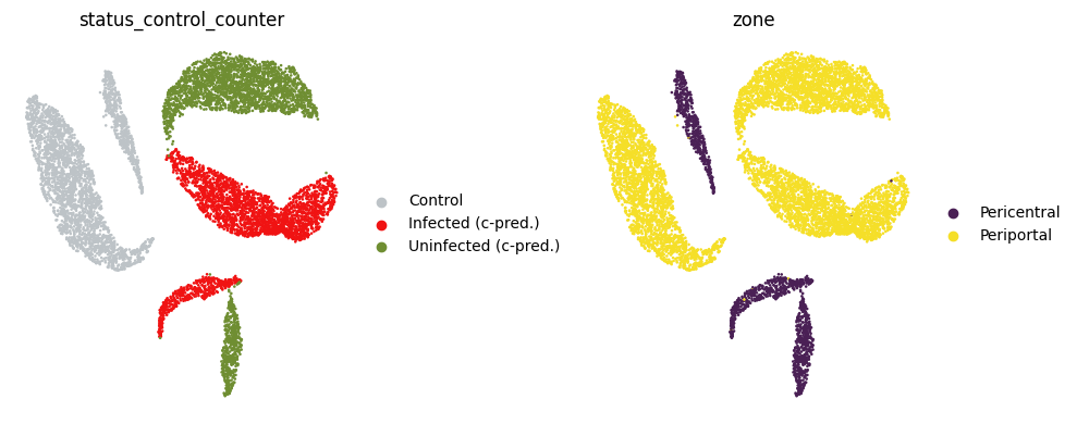
Visualize expression predictions

sc.pp.pca(adata_preds)
sc.pp.neighbors(adata_preds)
sc.tl.umap(adata_preds)

adata_preds.obs["status_control_counter"] = adata_preds.obs["status_control"].copy()
adata_preds.obs["status_control_counter"] = adata_preds.obs["status_control_counter"].cat.rename_categories(
    {"Infected": "Infected (c-pred.)", "Uninfected": "Uninfected (c-pred.)"}
)

adata_preds.uns["status_control_counter_colors"] = ["#bdc3c7", "#f01313", "#6f8e32"]

size = 4
fig, axs = plt.subplots(1, 2, figsize=(2 * (size + 1), size))

for i, c in enumerate(["status_control_counter", "zone"]):
    sc.pl.umap(adata_preds, color=[c], ax=axs[i], show=False)

    axs[i].set_axis_off()

plt.tight_layout()
plt.show()

Score genes

To find infection-related changes at the level of individual cells we use the dependent t-test for paired samples. Testing for the null hypothesis that the counterfactual predictions and original expressions have identical average (expected) values.

scores_genes_ttest = {}
for gene in adata_source.var_names:
    res = ttest_rel(
        a=adata_preds[adata_preds.obs["status_control"] == "Infected", gene].X,
        b=adata_preds[adata_preds.obs["status_control"] == "Control", gene].X,
    )

    scores_genes_ttest[gene] = {"statistic": res.statistic[0], "pvalue": res.pvalue[0]}

df_pvalue = pd.DataFrame.from_dict(scores_genes_ttest).T
df_pvalue.head()

	statistic	pvalue
A1bg	45.032546	0.000000e+00
A1cf	16.502016	1.639028e-58
A2ml1	79.963170	0.000000e+00
Aaas	41.639395	9.846481e-297
Aacs	-53.408096	0.000000e+00